Let’s IOT with Ruuvi & Atlas Stream Processing

Photo by Lisheng Chang on Unsplash

Bridging the gap between the physical world and the data sphere is always fun. It’s just a matter of deciding which device is the easiest and most useful to integrate. Luckily, Ruuvi has a sensor that lends itself perfectly to demonstrating the power of Atlas Stream Processing for an Internet of Things (IoT) use case. It costs about $50 and can be delivered via Amazon Prime quickly!

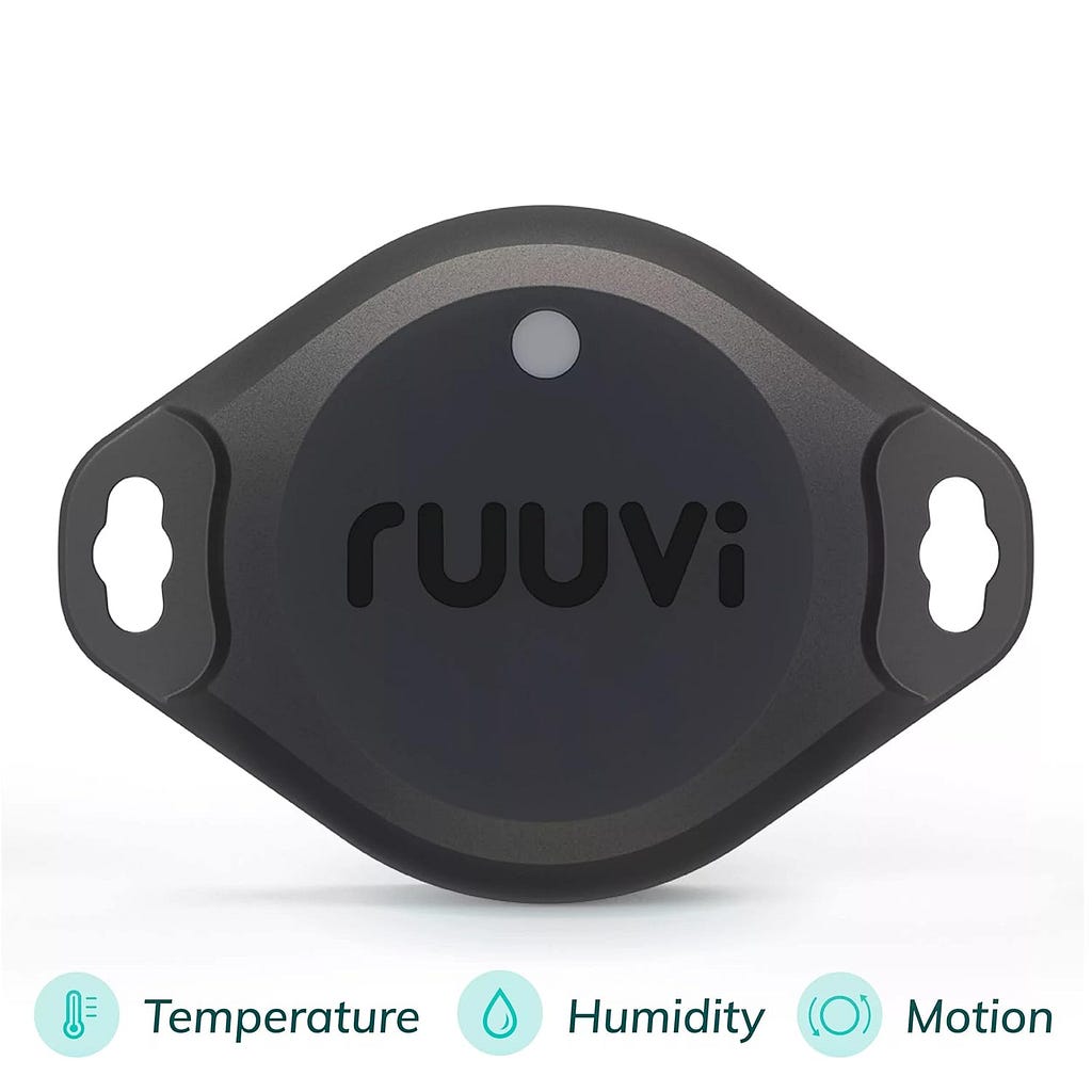
Temperature data processing has been done so many times before. Still, this little device also has an accelerometer built in, so let’s use that to create a streaming data pipeline for a motion detector with some cool graphs using Atlas Stream Processing and Atlas Charts.

Our streaming data pipeline will look like this:

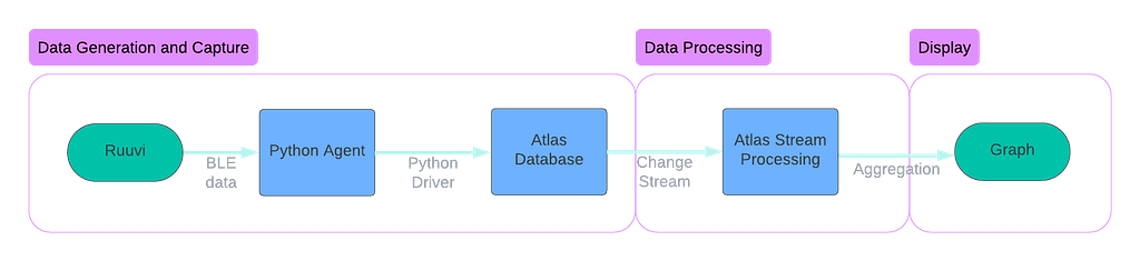
Data Generation and Capture

The Ruuvi device is a Bluetooth Low Energy (BLE) device. This wireless technology allows communication over short distances with low power requirements. In this example, we will grab the data from the sensor using our Mac laptop, which speaks over BLE directly to the sensor. Using the ruuvitag-sensor library on Github makes this easy. This gives us a data payload that looks something like this:

{  
    'data_format': 5,   
    'humidity': 44.95,   
    'temperature': 24.73,   
    'pressure': 987.62,   
    'acceleration': 980.163251708612,   
    'acceleration_x': 8,   
    'acceleration_y': -16,   
    'acceleration_z': 980,   
    'tx_power': 4,   
    'battery': 3178,   
    'movement_counter': 85,   
    'measurement_sequence_number': 40794,   
    'mac': 'cdc91fce729a',   
    'rssi': -55  
}

Next, we need to send this data to MongoDB Atlas for storage. We will use the native Python driver to write to an Atlas capped collection, and from there, we can read it as a change stream of events. For this example, we store the data in a MongoDB collection (we might use Apache Kafka to store this event log in a production setting). The code is straightforward — we add a timestamp (event time) to the data payload and then insert the document into the collection. Because we will be consuming the change stream only, we don’t need any indexing, and the _id field isn’t of great importance, so we use the default generated primary key.

# store data into MongoDB  
def store_data_in_mongo(mac_address, sensor_data):  
    utc_datetime = datetime.now(tz=timezone.utc)  
    document = {  
        'time': utc_datetime,  
        'mac_address': mac_address,  
        'data': sensor_data  
    }  
    try:  
        # insert into a collection  
        collection.insert_one(document)  
        print(f"Inserted sensor data from {mac_address} into MongoDB")  
    except Exception as e:  
        print(f"Error inserting data into MongoDB: {e}")

Data Processing

The raw data is now landing in the MongoDB database. But to aggregate that data into a motion detection graph, we need to process that data. Atlas Stream Processing was designed to do just this — take a raw stream of data, process that data through a pipeline, and return data for this purpose.

Atlas Stream Processing is based on the MongoDB aggregation language- so if you have been using MongoDB, you are automatically a stream processing engineer. The simple code defines an array of stages to process the data from source to sink, with any number of stages in between to mutate your stream until your heart is content.

// the anatomy of a simple Atlas Stream Processing Pipeline  
  
// define a source  
let source = {$source: { connectionName: 'cluster01', db: 'd1', coll: 'c1'}}  
  
// define other stages using MongoDB aggregation language   
let match = {$match: { age: 30, status: 'active' }}  
  
// define the sink stage  
let sink = {$emit: { connectionName: 'KafkaCluster', topic: 'mongoData'}}  
  
// define the pipeline, an array of stages in order  
let processor = [source, match, sink]  
  
// run the processor!  
sp.process(processor);

That is a simple processor. So, let’s get a bit more complicated by filtering and aggregating our sensor data. Let’s use this pattern to create a processor that handles the Ruuvi example. The key step in this processor is stage 4, where we take the max acceleration value over a 5-second period, which will indicate motion in our graph.

1. stage 1: create a source to read from the MongoDB change stream.
2. stage 2: pre-process the data to clean up its structure slightly.
3. stage 3: check for nulls and set to 0 if found
4. stage 4: create a tumbling window to aggregate the data over a 5-second window, accumulating accelerometer data as we go, computing the max value for the window period.
5. stage 5: further cleanse the data removing metadata we don’t need.
6. stage 6: create a sink to write the data to a cluster in aggregated form by primary key (mac address). This is an easy place for our graph to pick it up.

// stage 1, source data  
let s = {  
  $source: {  
    connectionName: "Cluster0",  
    db: "ruuvi_data",  
    coll: "sensor_data",  
  },  
};  
  
// stage 2, simple pre-processing, data cleaning  
let rr = { $replaceRoot: { newRoot: "$fullDocument" } };  
  
// stage 3, null handling  
let p = {  
  $project: {  
    mac_address: 1,  
    acceleration_num: {  
      $ifNull: ["$data.acceleration", 0],  
    },  
  },  
};  
  
// stage 4: aggregation  
let w = {  
  $tumblingWindow: {  
    interval: {  
      size: 5,  
      unit: "second",  
    },  
    pipeline: [  
      {  
        $group: {  
          _id: "$mac_address",  
          acceleration: {  
            $max: "$acceleration_num",  
          },  
        },  
      },  
    ],  
  },  
};  
  
// stage 5, cleaning metadata   
let pp = {  
  $project: {  
    _stream_meta: 0,  
  },  
};  
  
// stage 6, write the data into sensor_data_aggregated collection  
let m = {  
  $merge: {  
    into: {  
      connectionName: "Cluster0",  
      db: "ruuvi_data",  
      coll: "sensor_data_aggregated",  
    },  
    on: ["_id"],  
    whenMatched: "replace",  
    whenNotMatched: "insert",  
  },  
};  
  
  
// create the processor definition  
let processor = [s, rr, p, w, pp, m];  
  
// create the processor with a name  
sp.createStreamProcessor('ruuvi', processor);  
  
// start the processor  
sp.ruuvi.start();

Display

Next, we can use Atlas Charts to graph our data. We want two graphs: one that is the gauge of movement and the other a simple time series showing the accelerometer values over time.

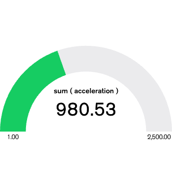
This graph shows when the sensor moves. As it sits on my desk, the motion of me typing this blog post is about 980, but if I shake the sensor, it spikes up to almost 30000.

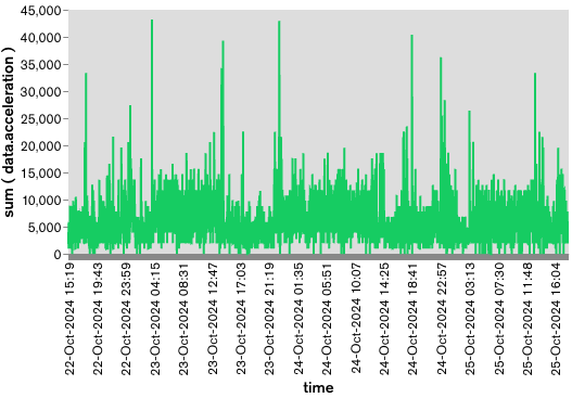
Lastly, our time series graph shows the data over time; you can see the brief spikes in motion as I move the sensor around or shake it. If you want the raw chart definitions, you can check them out here:

https://medium.com/media/55e6e0936858894a4c609e4df32b5a1b/href

If you want to try Atlas Stream Processing for yourself — you can go here:Atlas Stream Processing

Lastly, if you want the complete example, contribute, or you found a bug, feel free to submit a PR to the Github repo.

Let’s IOT with Ruuvi & Atlas Stream Processing was originally published in MongoDB on Medium, where people are continuing the conversation by highlighting and responding to this story.