Visualize fraudulent transactions via CEP with Kafka, Flink, SQL, D3.js and Mapbox.

I am not too proud to admit it — I like writing code in javascript. I’m a novice, but along with Python it’s my go-to language given a task at hand needing completion.

ObservableHQ.com describes itself as “Observable is a magic notebook for exploring data and thinking with code.” — and I tend to agree. Put another way, it’s javascript notebooks with D3. If you are familiar with D3.js and javascript, but want to have the usability and exploration characteristics of a notebook (think Jupyter), then Observable is for you. In this example, I will be using synthetic Kafka data generated via the Eventador Examples repo, and will be pulling that data into Observable and using it to create a heatmap of fraudulent transactions using Complex Event Processing in SQL.

Let’s get into it. Detailed instructions are in the repo, I will cover the highlights here.

First let’s build a streaming data pipeline

In this example, I assume you are using the Eventador Platform and Continuous SQL to identify fraudulent transactions via CEP, then we visualize them in the notebook. First I generate fake transactions (including fraudulent ones) via a python script running in a docker container:

git clone git@github.com:Eventador/eventador_examples.git
cd eventador_examples/fraud
docker build . -t fraud
docker run -d --env-file fraud.env fraud

This generates JSON data in the form:

{
 "userid": 256,
 "amount": 39101,
 "lat": 30.378,
 "lon": -97.448,
 "card": "4921156448685188"
}

And we need to process this stream of data looking for patterns over time. Complex Event Processing is supported in SQL via the match_recognize syntax, and is run via Eventador SQLStreamBuilder on Apache Flink:

SELECT *
FROM authorizations
MATCH_RECOGNIZE(
  PARTITION BY card
  ORDER BY eventTimestamp
  MEASURES
      A.amount AS start_amount,
      A.eventTimestamp AS first_timestamp,
      A.lat AS lat,
      A.lon AS lon,
      B.amount AS next_amount,
      B.eventTimestamp AS next_timestamp,
      C.amount AS finish_amount,
      C.eventTimestamp AS finish_timestamp
  ONE ROW PER MATCH
  AFTER MATCH SKIP PAST LAST ROW
  PATTERN (A B C)
  WITHIN INTERVAL '1' MINUTE
  DEFINE
    A AS A.amount IS NOT NULL
      AND CAST(A.amount AS integer) >= 0
      AND CAST(A.amount AS integer) <= 1000,
    B AS B.amount IS NOT NULL
      AND CAST(B.amount AS integer) >= 1001
      AND CAST(B.amount AS integer) <= 2000,
    C AS C.amount IS NOT NULL
      AND CAST(C.amount AS integer) > 2001)

Our pattern for finding fraud is defined in the SQL statement as (not in order of execution):

• Get everything from the authorizations virtual table (defined in Eventador: a topic with schema)
• Partition your search by card (the card #)
• Return one row per match, if matched, finish
• Don’t run in greedy mode (must match each step)
• Over a 1 minute interval the card # must be ≥ 0 ≤ 1000 then ≥ 1001 and ≤ 2000 and then > 2001
• Order results by timestamp
• Return amounts at each stage, timestamp at each stage, and lat/lon of first stage

I materialize the results and present them over a RESTful endpoint so we can map them. Again, this complexity is provided as part of the Eventador Platform. Ultimately all I need to know from an ObservableHQ notebook perspective is the URL of the endpoint.

Copy the URL of the REST endpoint, we will use it below.

Next, let’s visualize the pipeline

This is where the notebook interface really shines. It’s extremely easy to utilize javascript and the D3 libraries to make excellent visualizations. For this example, we will be using the Mapbox GL JS API inside an Observable notebook. This takes just 4 cells.

We need a couple of functions to help us out. The first step is to create a cell with an object for the GL libraries, you need to pass your access token in this function. Change <mytoken> to your token.

mapboxgl = {
  const gl = await require("mapbox-gl@0.49");
  if (!gl.accessToken) {
    gl.accessToken = "<mytoken>";
    const href = await require.resolve("mapbox-gl@0.49/dist/mapbox-gl.css");
    document.head.appendChild(html`<link href=${href} rel=stylesheet>`);
  }
  return gl;
}

Next, we need a cell with a function to translate the raw JSON results to geoJSON:

function to_geojson(d){
  var features = [];
  for (var i in d) {
    var feature = {
      "type": "Feature",
      "geometry": {
        "type": "Point",
        "coordinates": [parseFloat(d[i].lon), parseFloat(d[i].lat), 0]
      },
      "properties": {
        "name": d[i].card
      }
    }
    features.push(feature);
  }
  var doc = {
    "type": "FeatureCollection",
    "features": features
  }
  return doc;
}

Let’s initialize D3 in another cell:

d3 = require("d3@5")

Now we can create the map. You will need to change <myRESTURL> to the REST endpoint we copied from the Eventador Platform.

viewof centerpoint = {
  let container = html`<div style='height:400px;' />`;
  yield container;
  let map = new mapboxgl.Map({
    container: container,
    center: [-104.84, 39.51],
    zoom: 8,
    style: "mapbox://styles/mapbox/navigation-guidance-night-v4"
  });
  map.on('load', function() {
    window.setInterval(function() {
      console.log("fetching data..")
      d3.json("<myRESTURL>")
        .then(function(data) {
          try {
            map.removeLayer('mylayer');
            map.removeSource('testme');
          } catch(err) {
            console.log(err);
          }
          map.addSource('testme', {
            'type': 'geojson',
            'data': to_geojson(data)
          });
          map.addLayer({
            'id': 'mylayer',
            'type': 'heatmap',
            'source': 'testme'
          });
        });
    }, 2000);
  });
}

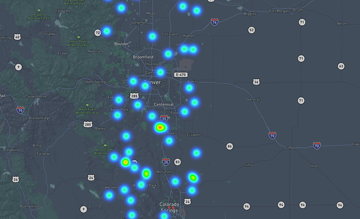
And we get a nice interactive heatmap using Mapbox. In this case, the metro Dallas, Austin, and Denver areas. You can check out the entire notebook here.